Selective Supervised Contrastive Learning with Noisy Labels

Contrastive Learning is able to learn good latent representations that can be used to achieve high performance in downstream tasks. Supervised contrastive learning enhances the learned representations using supervised information. However, noisy supervised information corrupts the learned representations. In this blog post, I will summarize the paper published in CVPR 2022 that proposes an algorithm to learn high quality representations in existence of noisy supervised information. The title of this paper is Selective Supervised Contrastive Learning with Noisy Labels.

A brief on contrastive learning

Contrastive learning (Con) aims to learn representations in a latent space that are closer to each other for similar examples and are far from each other for dissimilar examples [1]. The advantage of Con algorithms is that by first learning good latent representations from an unlabeled dataset, they can learn a downstream task with high performance using a small labeled portion of the dataset. While training the Con network, pairs of examples are fed to the network. Originally, only one similar pair (positive pair) and one dissimilar pair (negative pair) were fed to the network. Recently, the proposed algorithms feed the network with a batch that includes multiple positive and negative pairs.

Why supervised contrastive learning?

Since there exists no labels when training the Con algorithm with an unlabeled dataset, a positive pair is generated by pairing a randomly selected example and an augmentation of the same example. Negative pairs are generated by pairing an example with any other example in the training dataset. Fasle negative pairs generated by samples from the same class can degrade the learned representations [2]. Using label information, positive pairs can be generated by pairing examples from the same class and negative examples can be generated by pairing examples from different classes. By providing better positive and negative pairs, the Con algorithm learns better latent repsentations.

In supervised Con (Sup-Con) [3], two augmentation operations are applied to each example in the input batch of data to generate two different views. Both views are passed through an encoder network and the output representations are L2-normalized. Positives for an example consist in the representations that correspond to the same example in the batch or to any other example in the batch with the same label. Negatives for an example are all the remaining examples in the batch. The representations are passed through a projection network as is common in Con algorithms to learn meaningful features. A supervised contrastive loss is imposed on the normalized outputs of the projection network [4]. Koshla et al. [3] show that Sup-Con consisently outperforms supervised learning.

How to handle noisy labels?

The proposed algorithm by the paper Selective Supervised Contrastive Learning with Noisy Labels [5] denoted by Sel-Con consists of two steps:

• Select pairs of examples that the algorithm is confident about their label.
• Train the network with the confident pairs using Sup-Con algorithm.

In the following, I will explain how the confident pairs are selected and are used to train the network. First, we need to find the confident examples.

How to find confident examples?

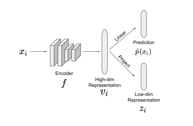
The noisy labeled dataset with $C$ different classes is denoted by \(\tilde{D} = \{(x_i, \tilde{y}_i)\}_{i=1}^n\) where $n$ is the number of examples in the training dataset, $x_i$ is the $i^{th}$ example and $\tilde{y}_i\in [C]$ is the corresponding noisy label. Figure shows the architecture of the Sel-Con network in the paper. Each example is passed through an encoder, $f$, to get a high-dimensional representation of the example denoted by $v_i$. A classifier head receives $v_i$ and outputs a class prediction shown by $\hat{p}(x_i)$. A linear or non-linear projection head maps $v_i$ to a lower dimensional representation $z_i$.

Confident examples are found by first measuring cosine distance between the low dimensional representations $z_i$, $z_j$ of each pair of examples as shown below:

They create a pseudo-label $\hat{y}_i$ for each example ($x_i$, $\tilde{y}_i$) by aggregating the original label from its top-k neighbors shown by \(\mathcal{N}_i\) with the lowest cosine distance:

and use the pseudo-labels to approximate the clean class psoterior probabilities. The set of confident examples belonging to the c-th class is denoted by $\mathcal{T}_c$ and is defined as:

where $\mathcal{l}$ refers to cross-entropy loss and $\gamma_c$ is a threshold for c-th class. $\gamma_c$ is set in a way to get a class-balanced set of confident examples. The confident example set for all classes is then defined as $\mathcal{T} = \bigcup_{c=1}^C \mathcal{T}_c$

How to select confident pairs?

The confident examples are transformed into a set of confident pairs by finding the union of two different sets. The first set is defined as shown below:

Where $P_{ij}$ is the pair built by the examples $(x_i,\tilde{y}_i)$ and $(x_j, \tilde{y}_j)$. This set consists of all possible pairs of examples from $\mathcal{T}$ with the same label. The second set is defined on the whole training dataset as:

Where $\tilde{s}_{ij} = \mathbb{I}[\tilde{y}_i = \tilde{y}_j]$ and $\gamma$ is a dynamic threshold to control the number of identified confident pairs. This set also includes examples that are misclassified to the same class. Later, in Eq. (8) and (10) you will see how such pairs (without their label) can be helpful to learn good latent representations. The final set of confidents pairs is defined as:

How is the network trained?

Following Sup-Con, instances are randomly selected in each mini-batch and two random data augmentation operations are applied to each instance generating two data views. The resulting training mini-batch data is \(\{(x_i,\tilde{y}_i)\}_{i=1}^{2N}\) where \(i \in I = [2N]\) is the index of an augmented instance. The network is trained using three losses. The first loss uses the Mixup technique [6] which generates a convex combination of pairs of examples as $x_i = \lambda x_a + (1-\lambda)x_b$, where $\lambda \in [0,1] \sim Beta(\alpha_m, \alpha_m)$; and $x_a$ and $x_b$ are two mini-batch examples. The label for the mixed example is either $\tilde{y}_a$ or $\tilde{y}_b$ and is identified by $\lambda$. The Mixup loss is defined as:

where $\mathcal{L}_a$ and $\mathcal{L}_b$ have the same form as Sup-Con loss that is defined as:

$A(i)$ specifies the set of indices excluding $i$ and \(\mathcal{G}_i = \{g\mid g \in A(i), P_{i'j'} \in \mathcal{G}\}\) where $i’$ and $g’$ are the original indices of $x_i$ and $x_g$ in $\tilde{D}$. Also, $\tau \in \mathbb{R}^+$ is a temperature parameter. Mixup loss helps learn robust representations. The second loss is a classfication loss and is applied on the confident examples. This loss is defined to stablize converegence and achieve better representations. The classification loss is defined as:

where $x_i$ can refer to the augmented image. Finally, inspired by recent methods [7,8], the authors add the third loss that trains the classifier with similarity labels ($\tilde{s}_{i,j}$) on the mini-batch data \(\{(x_i, \tilde{y}_i)\}_{i=1}^{2N}\). The similarity loss is:

The algorithm uses unsupervised training to initially train the network in the first few epochs. Once confident pairs are identificed, the network is trained using the overall loss below:

where $\lambda_c$ and $\lambda_s$ are loss weights. The confident pairs are iteratively identified and are used to learn robust representations at each epoch. As a result, better confident pairs will result in better learned representations and better representations will identify better confident pairs. For other examples, unsupervised Con is used.

The proposed algorithm is evaluated on simulated noisy datasets generated by injecting different levels of noise on CIFAR10/100 datasets as well as a real-world noisy dataset: WebVision. For the sake of keeping this blog post short, I did not summarize the evaluation results here. To see the evaluation results please refer to the paper.

References

[1] Van den Oord, et al. “Representation learning with contrastive predictive coding.” arXiv e-prints (2018): arXiv-1807.

[2] Chuang, Ching-Yao, et al. “Debiased contrastive learning.” Advances in neural information processing systems 33 (2020): 8765-8775.

[3] Khosla, Prannay, et al. “Supervised contrastive learning.” Advances in Neural Information Processing Systems 33 (2020): 18661-18673.

[4] Google Blog: https://ai.googleblog.com/2021/06/extending-contrastive-learning-to.html?m=1

[5] Li, Shikun, et al. “Selective-Supervised Contrastive Learning with Noisy Labels.” arXiv preprint arXiv:2203.04181 (2022).

[6] Zhang, Hongyi, et al. “mixup: Beyond empirical risk minimization.” arXiv preprint arXiv:1710.09412 (2017).

[7] Hsu, Yen-Chang, et al. “Multi-class classification without multi-class labels.” arXiv preprint arXiv:1901.00544 (2019).

[8] Wu, Songhua, et al. “Class2simi: A new perspective on learning with label noise.” (2020).