
Using Radiomics for Tree Bark Identification
Published:
Using Radiomics for Tree Bark Identification
Since the term was first coined in $2012$, Radiomics has widely been used for medical image analysis. Radiomics refers to the automatic or semi-automatic extraction of a large of number of quantitative features from medical images. These features have been able to uncover characteristics that can differentiate tumoral tissue from normal tissue and tissue at different stages of cancer.
In this blog, we aim to show that Radiomic features can be useful for analysis of images in many other domains. The example we have provided here shows that radiomic features can be used for tree bark identification. We use Trunk12, a publicly available dataset of tree bark images from here. The code for this blog is available at this link.
Trunk12 Dataset
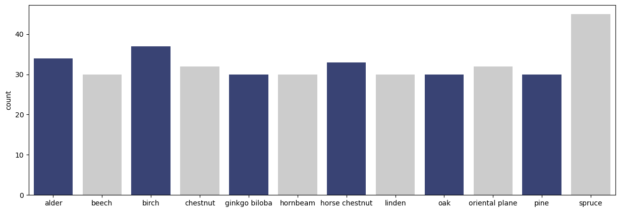
Trunk12 consists of $393$ RGB images of tree barks captured from $12$ types of trees in Slovenia. For each type of tree, there exists about $30$ jpeg images of resolution $3000 \times 4000$ pixels. The images are taken using the same camera Nikon COOLPIX S3000 and while following the same imaging setup: same distance, light conditions and in an upright position. The following chunk of code plots the number of images in each class in this dataset:
import torchvision
import seaborn as sns

# Location of the dataset
data_dir = '../data/trunk12'

# Read images from the dataset directory
dataset = torchvision.datasets.ImageFolder(root=data_dir)

# Show the number of images in each class
plt.figure(figsize=[15, 5])
p = sns.countplot(dataset.targets, palette=['#2F3C7E', '#CCCCCC'])
p.set_xticklabels(dataset.classes);
The number of images in each class are shown below.
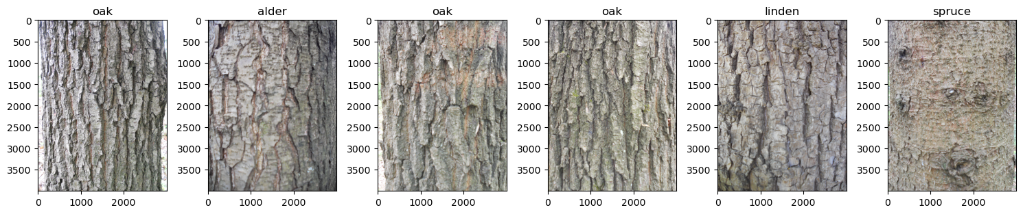
We also show a few examples of images in this dataset together with their tree type using the code below.
import torchvision.transforms as transforms
import matplotlib.pyplot as plt
from PIL import Image
import random
import torch

n = 6
indices = random.sample(range(0, len(dataset.imgs)),n)
batch = [dataset.imgs[i] for i in indices]
trans = transforms.ToTensor()

plt.figure(figsize=[15,5])
for i in range(n):
    img = Image.open(batch[i][0])
    img = trans(img)
    img = torch.permute(img, (1,2,0))
    target = dataset.classes[batch[i][1]]
    plt.subplot(1,n,i+1)
    plt.imshow(img)
    plt.title(target)
plt.tight_layout()
plt.show()
The output of this code is shown in the following figure:
To prepare this dataset for radiomic feature extraction we perform a few preprocessing steps on the images. These steps are explained in the following section.
Preprocessing
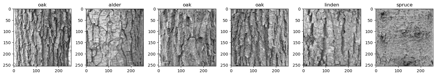
All images go throught the following preprocessing steps. First, the images are converted to grayscale. Second, squares of size $3000 \times 3000$ pixels are cropped from the center of images. Third, the cropped squares are downsampled to the size $250 \times 250$ pixels. Finally, image contrast is increased so that the intensity values in each image coveres the range $[0,255]$. The preprocessing code is provided below:
import numpy as np
import nibabel as nib
from PIL import Image, ImageOps
import os

crops_s = 3000
new_s = 256
half_crop_s = int(crop_s/2)

for file, label in dataset.imgs:

    # Open an image
    img = Image.open(file)

    # Convert it to a grayscale image
    img = ImageOps.grayscale(img)

    # Down-sample the image
    w2 = int(img.size[0]/2)
    h2 = int(img.size[1]/2)
    img = img.crop((w2-half_crop_s, h2-half_crop_s, w2+half_crop_s, h2+half_crop_s))
    img = img.resize((new_s,new_s))

    # Increase contrast of the image
    extrema = img.getextrema()
    arr = np.asarray(img).astype('float')
    arr = (arr - extrema[0])/ (extrema[1] - extrema[0]) * 255

    # Write the image ...
Below, we show the same images that were shown above after going through these preprocessing steps.
In the next step, we extract Radiomic features from the processed images. But first we provide a brief introduction on Radiomic features.
What are Radiomic Features?
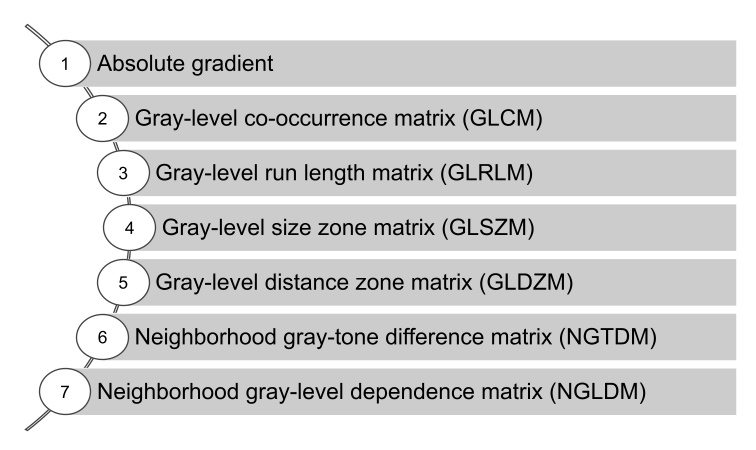
Radiomics is quantifying and extracting many imaging patterns including texture and shape features from images using automatic and semi-automatic algorithms. These features, usually invisible to the human-eye, can be extracted non-subjectively and used to train and validate models for prediction and early stratification of patients. Radiomic features are categorized into five groups of features.
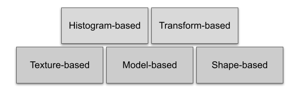
These features are extracted from the region of interest in an image which is specified by a mask. We will give a brief explanation for each family of features:
Histogram-based features: These are the group of quantitative features that can be extracted from the histogram of the intensity values for the region of interest in the image. Examples of these features include mean, max and min intensity values, variance, skewness, entropy and kurtosis.
Transform-based features: Tranform-based features are features that are extracted after transfering the region of interest to a different space by applying a transformation function. Such transformation functions include Fourier, Gabor and Harr wavelet transform. Quantitative features such as histogram-based features are extracted from the transformed region of interest.
Texture-based features: These features aim to extract quantitative features that represent variations in the intensities within the region of interest. Examples of features in this family of features are:
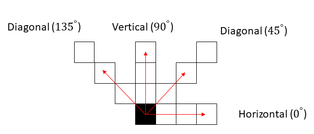
Extracting any of these features first requires specifying the direction of extraction. Any of the following directions can be selected:
As an example, extracting GLCM in the horizontal direction from a region of interest outputs a matrix. Elements of this matrix specify the number of times different combination of intensity values occur in the region of interest horizontally.
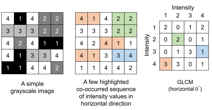
As can be seen, GLCM is not a quantitative feature per-se but quantitative features are extracted from GLCM. Some of the quantitative features that can be extracted from GLCM are shown in the table below:
| Texture Matrix | Features | Description |
|---|---|---|
| GLCM | Contrast | Measures the local variations in the GLCM. |
| Correlation | Measures the joint probability occurrence of the specified pixel pairs. | |
| Energy | Provides the sum of squared elements in the GLCM. Also known as uniformity or the angular second moment. | |
| Homogeneity | Measures the closeness of the distribution of elements in the GLCM to the GLCM diagonal. |
Model-based features: Parameterised models such as autoregressive models or fractal analysis models can be fitted on the region of interest. Once the parameters for these models are estimated, they are used as Radiomics features.
Shape-based features: Shape-based features describe geometric properties of the region of interest. Compactness, sphericity, density, $2$D or $3$D dimeters, axes and their ratios are examples of features in this family.
Now that we have a better idea what Radiomics features are, we will proceed with extracting these features from our processed tree bark images.
Radiomic Feature Extraction
To extract Radiomics features from our dataset of tree bark images we take advantage of the PyRadiomics library. This library can extract up to $120$ radiomic features (both $2$D and $3$D). One limitation of PyRadiomics is that it is developed for medical images so it can only extract features from medical images with file formats such as NIfTI, NRRD, MHA, etc. These file formats usually have a header which contains information about the patient, acquisition parameters and orientation in space so that the stored image can be unambigiuosly interpreted. To address this problem, we converted our jpeg images to NIfTI images using the following hack:
import nibabel as nib
from PIL import Image
import numpy as np

# Location of the dataset
data_dir = '../data/trunk12'

# Location where NIfTI images are written
nii_dir = f'../data/trunk12_nii'

# Open a jpeg image and write it in NIfTI format
img = Image.open(jpg_filename)
arr = np.asarray(img).astype('float')
arr = np.expand_dims(arr, axis=2)
empty_header = nib.Nifti1Header()
affine =  np.eye(4)
nifti_img = nib.Nifti1Image(arr, affine, empty_header)
nifti_filename = jpg_filename.replace(data_dir, nii_dir)
nifti_filename = nifti_filename.replace('.JPG', '.nii.gz')
path = nifti_filename.replace(nifti_filename.split('/')[-1], "")
os.makedirs(path, exist_ok = True)
nib.save(nifti_img, nifti_filename)
As can be seen, we have defined an empty header with an identity matrix for the affine transform matrix. The affine transform matrix gives the relationship between pixel or voxel coordinates and world coordinates. The same header and affine transform matrix is defined for all jpeg images in our dataset. As a result, the extracted Radiomic features from these images are comparable. PyRadiomics also requires a mask file that specifies the region of interest to extract features from in the input image. For our case, we plan to extract features from the entire image. Therefore, we generate a mask file that covers almost the whole image as shown below. The reason we don’t set the mask to cover the whole image is that PyRadiomics currently doesn’t support this.
import nibabel as nib
from PIL import Image
import numpy as np

# Write a mask file in NIfTI format
mask = np.ones(img.shape) *255
mask[:1, :1, :] = 0
mask = mask.astype(np.uint8)
mask_filename = "../outputs/mask.nii.gz"

empty_header = nib.Nifti1Header()
affine = np.eye(4)
mask_img = nib.Nifti1Image(mask, affine, empty_header)
nib.save(mask_img, mask_filename)
Above, we specified the label for the region of interest with $255$. Now, we can extract Radiomic features from the generated NIfTI images using the mask file and the label as shown in the following:
import radiomics
from radiomics import featureextractor

# Instantiate the radiomics feature extractor
nifti_filename = dataset.imgs[0][0].replace(data_dir, nii_dir).replace('.JPG', '.nii.gz')
extractor = featureextractor.RadiomicsFeatureExtractor(force2D=True)
output = extractor.execute(nifti_filename), mask_filename, label=255)
Figure below shows the extracted features by PyRadiomics and their values from an image in our dataset:
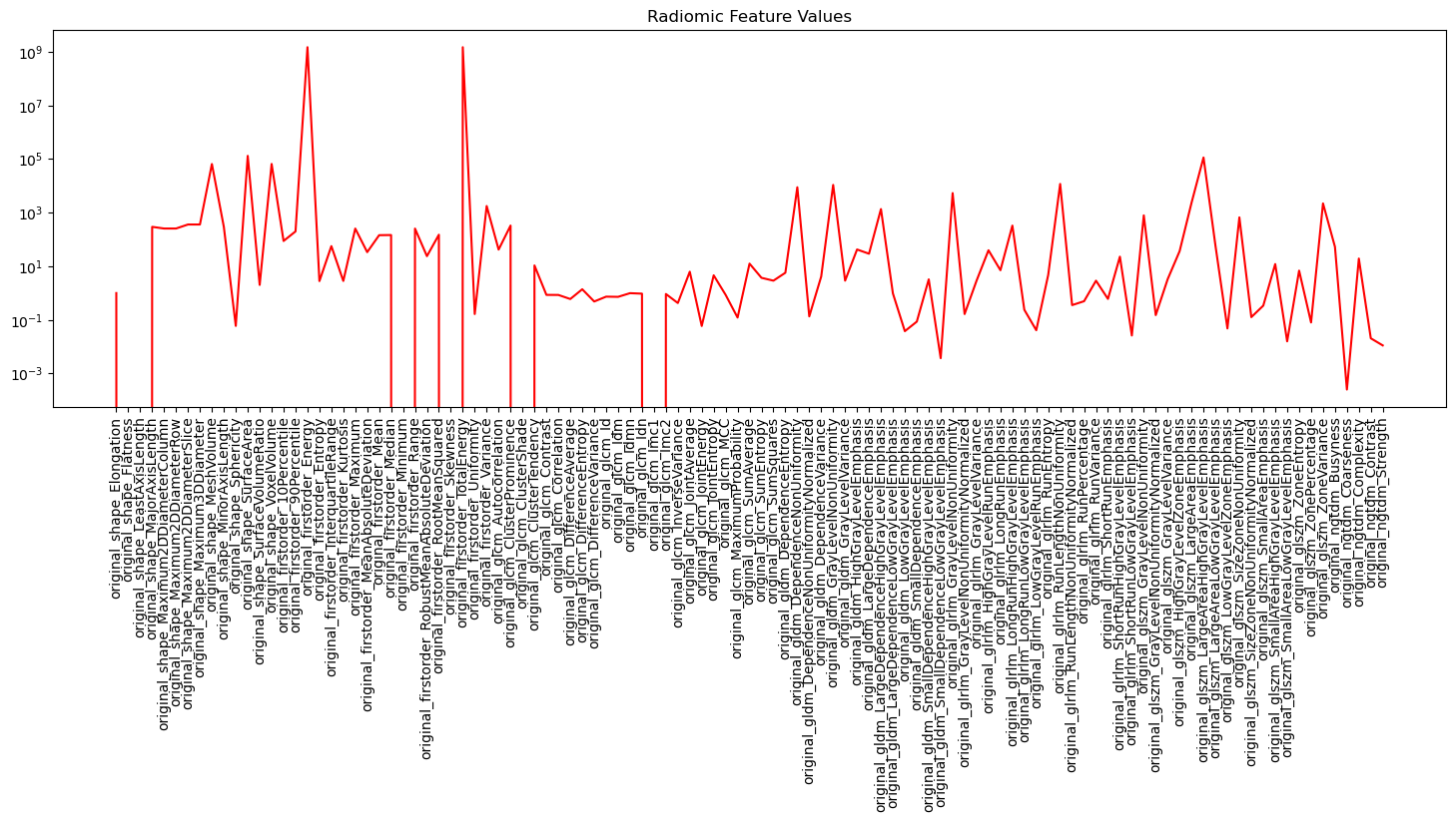
As shown, the range of feature values is between $0$ and $10^9$. To extract radiomic features from all images in our dataset, we can generate an excel sheet that contains the location of all the NIfTI images in our dataset together with the mask file and label and pass this excel sheet to PyRadiomics for feature extraction. The same mask file and label is used for all images. Below we show how the excel sheet is generated:
import csv
import numpy as np
import pandas as pd

# Write a csv file that contains the location of each NIfTI image in the train set, its mask file and label
pyradiomics_header = ('Image','Mask', 'Label')
m_arr = [mask_filename] * len(dataset.imgs)
rows = [(i[0].replace(data_dir, nii_dir).replace('.JPG', '.nii.gz'), m, 255) for m, i in zip(m_arr, dataset.imgs)]
rows.insert(0, pyradiomics_header)
arr = np.asarray(rows)
np.savetxt('../outputs/pyradiomics_samples.csv', arr, fmt="%s", delimiter=",")
Next, this excel sheet is passed as input to PyRadiomics as shown below:
# Run Pyradiomics on pyradiomics_sample.csv, output to pyradi_features_3000_256.csv
!pyradiomics -o ../outputs/pyradi_features_{crop_s}_{new_s}.csv -f csv ../outputs/pyradiomics_samples.csv &> ../outputs/log.txt
This command will generate another excel sheet named pyradi_features_$3000$_$256$.csv which contains at each row the Radiomic feature values for each image in the pyradiomics_samples.csv file.
Radiomic Feature Processing
The output feature values are saved in the file pyradi_features_$3000$_$256$.csv for each image in the dataset. Now, we can open this file and have a look at it. The first 25 columns in this file contain information about parameters that were used for feature extraction. The rest of the columns contain the extracted features. This is a total of $107$ Radiomic features for our dataset.
import pandas as pd

# Declare csv filename from Pyradiomics (zscore scaled and merged)
fname = f'../outputs/pyradi_features_{crop_s}_{new_s}.csv'

# Load data
pyradi_data = pd.read_csv(fname)

# Show the radiomic feature columns
pyradi_original = pyradi_data.iloc[:,25:]
pyradi_original.head()
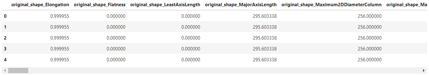
As shown above, the shape feature values have the same values. This is because the region of interest is the same for all images. To train a classifier on the Radiomic features, we first need to normalize the feature values to the range $[0,1]$ and remove those feature columns with nan values using the code below. Also, we add the tree types as the class labels to the excel sheet.
# Normalize the feature values
pyradi_original_norm = (pyradi_original - pyradi_original.min()) / (pyradi_original.max() - pyradi_original.min())

# Add the class labels
pyradi_original_norm['target'] = dataset.targets

# Drop features will NaN values
pyradi_original_norm = pyradi_original_norm.dropna(axis=1, how='all')
Removing features with nan values after normalization reduces the number of Radiomic features to $90$. Next, we proceed with training different classifiers on these features.
Training Classifiers
We define a function called evaluate_model that trains and evaluates an input model on the input dataset using k-fold cross validation. This function measures precision, recall, accuracy and F$1$ score as the evaluation metrics for the input model and dataset. This function is defined below:
from sklearn.metrics import precision_score
from sklearn.metrics import recall_score
from sklearn.metrics import roc_curve
from sklearn.metrics import roc_auc_score
from sklearn.model_selection import StratifiedKFold
from sklearn.metrics import accuracy_score
from sklearn.metrics import f1_score
from sklearn.pipeline import make_pipeline
import statistics
from sklearn.metrics import matthews_corrcoef

# Function to evaluate a classification model using k-fold cross validation
def evaluate_model(model, df, y, calc_auc=False):
    auc_lr=[]
    pre_lr=[]
    rec_lr=[]
    acc_lr=[]
    f1_lr=[]
    auc_lrt=[]
    pre_lrt=[]
    rec_lrt=[]
    acc_lrt=[]
    f1_lrt=[]

    cv = StratifiedKFold(n_splits=7,  shuffle=False)
    for train_index, test_index in cv.split(df, y):

       # Get a fold
        X_train, X_test = df.iloc[train_index], df.iloc[test_index]
        Y_train, Y_test= y.iloc[train_index], y.iloc[test_index]

        X_train= X_train.values
        X_test= X_test.values
        Y_train= Y_train.values
        Y_test= Y_test.values

	  # train the model
        clf = make_pipeline(model)
        clf.fit(X_train, Y_train)

        # Get predictions and measure evaluation metrics for the trained model
        pred = clf.predict(X_test)
        pre_l = precision_score(Y_test, pred, average='weighted')
        rec_l = recall_score(Y_test, pred, average='weighted')
        acc_l = accuracy_score(Y_test, pred)
        if calc_auc:
            probs = clf.predict_proba(X_test)
            auc_l = roc_auc_score(Y_test, probs, average='weighted', multi_class='ovr')

        f1_l = f1_score(Y_test, pred, average='weighted')

        pred = clf.predict(X_train)
        pre_lt = precision_score(Y_train, pred, average='weighted')
        rec_lt = recall_score(Y_train, pred, average='weighted')
        acc_lt = accuracy_score(Y_train, pred)
        if calc_auc:
            probs = clf.predict_proba(X_train)
            auc_lt = roc_auc_score(Y_train, probs, average='weighted', multi_class='ovr')
        f1_lt = f1_score(Y_train, pred, average='weighted')

        # Keep the evaluation metric values for each fold
        if calc_auc: auc_lr.append(auc_l)
        pre_lr.append(pre_l)
        rec_lr.append(rec_l)
        acc_lr.append(acc_l)
        f1_lr.append(f1_l)

        if calc_auc: auc_lrt.append(auc_lt)
        pre_lrt.append(pre_lt)
        rec_lrt.append(rec_lt)
        acc_lrt.append(acc_lt)
        f1_lrt.append(f1_lt)

    # Measure the average of the evaluation metrics for all the folds
    avg_auc_lrt = -1
    avg_pre_lrt = statistics.mean(pre_lrt)
    avg_rec_lrt = statistics.mean(rec_lrt)
    avg_acc_lrt = statistics.mean(acc_lrt)
    if calc_auc: avg_auc_lrt = statistics.mean(auc_lrt)
    avg_f1_lrt = statistics.mean(f1_lrt)

    avg_auc_lr = -1
    avg_pre_lr = statistics.mean(pre_lr)
    avg_rec_lr = statistics.mean(rec_lr)
    avg_acc_lr = statistics.mean(acc_lr)
    if calc_auc: avg_auc_lr = statistics.mean(auc_lr)
    avg_f1_lr = statistics.mean(f1_lr)

    return avg_pre_lrt, avg_rec_lrt, avg_acc_lrt, avg_auc_lrt, avg_f1_lrt, avg_pre_lr, avg_rec_lr, avg_acc_lr, avg_auc_lr, avg_f1_lr
For instance, to test a SVM classifier on our dataset we run the following code:
from sklearn.svm import SVC

# Get the class labels and drop the class column
Y = pyradi_original_norm['target']
pyradi_original_norm = pyradi_original_norm.drop('target', axis=1)

# Evaluate an SVM classifier
calc_auc = True
model = SVC(kernel='poly', degree=4, probability=True)
stats_svc = evaluate_model(model, pyradi_original_norm, Y, calc_auc)

print("---------------TRAIN---------------")
print("PRE:\t %.02f"% stats_svc[0])
print("REC:\t %.02f"% stats_svc[1])
print("ACC:\t %.02f"% stats_svc[2])
if calc_auc: print("AUC:\t %.02f"% stats_svc[3])
print("F1:\t %.02f"% stats_svc[4])

print("---------------TEST---------------")
print("PRE:\t %.02f"% stats_svc[5])
print("REC:\t %.02f"% stats_svc[6])
print("ACC:\t %.02f"% stats_svc[7])
if calc_auc: print("AUC:\t %.02f"% stats_svc[8])
print("F1:\t %.02f"% stats_svc[9])
This code prints the measured evaluation metrics for the SVM classifier on tree bark images for training and test data. Now, we compare different classifiers using these evaluation metrics.
Evaluation Results
We tested multiple models including XGBoost, SVM and Random Forest on our dataset and compared our results with the results of the paper (Boudra et al, $2018$) for this dataset in the table below. Boudra et al. propose a novel texture descriptor and use this descriptor to guide classification of tree bark images. We first plot the precision-recall curve for each tested model as shown below:
| XGBoost | SVM | Random Forest |
|---|---|---|
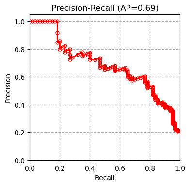 | 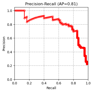 | 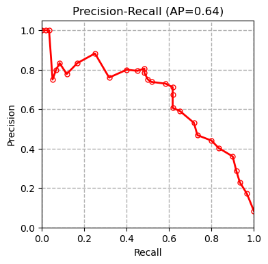 |
| Logistic Regression | SGD | Boudra et al. 2018 |
|---|---|---|
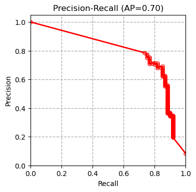 | 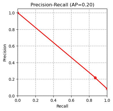 | 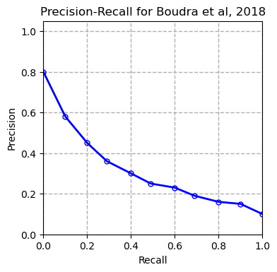 |
AP refers to average precision. The measurements are done using micro averaging. The precision-recall curves show that the SVM classifier outperforms all the other methods. Other evaluation metrics measured by the evaluate_model function also confirm this conclusion.
| Classifier | XGBoost | SVM | Random Forest | Linear Regression | SGD | Boudra et al. (2018) |
|---|---|---|---|---|---|---|
| Precision | 0.660 | 0.703 | 0.603 | 0.680 | 0.513 | - |
| Recall | 0.656 | 0.699 | 0.603 | 0.679 | 0.501 | - |
| Accuracy | 0.656 | 0.699 | 0.603 | 0.679 | 0.501 | 0.677 |
| AUC | 0.935 | 0.953 | 0.914 | 0.950 | 0.751 | - |
| F1 | 0.638 | 0.682 | 0.580 | 0.663 | 0.445 | - |
All measurements are done using weighted averaging.
Conclusion
In this blog, we showed that Radiomics analysis can be as useful in other areas as in medical domain. As an example, we showed how Radiomic features can help classify tree bark images. We used PyRadiomics library to extract Radiomic features from the Trunk12 dataset. Although this library can only work with medical image file formats, we showed how we can hack our way through by converting our jpeg images to NIfTI images. We then trained multiple classifiers on the extracted Radiomic features from these NIfTI images and compared their performance. Our analysis showed that training a SVM classifier on Radiomic features extracted from tree bark images gives the highest classification performance compared to other classifiers trained on the same Radiomic features and a different approach proposed by Boudra et al. (2018).
One topic that is important but not covered in this blog is feature selection. Many times, using ony a few carefully selected Radiomic features have more predictive capability than using all the extracted features. Although, using all the Radiomic feature resulted in the highest classification performance in the example in this blog, it is worth considering different feature selection methods in your projects instead of passing all the Radiomic features to your classifier.
Reference
Boudra, S., Yahiaoui, I., & Behloul, A. (2018, September). Bark identification using improved statistical radial binary patterns. In 2018 International conference on content-based multimedia indexing (CBMI) (pp. 1-6). IEEE.